How accurate is the simulation?
Like the Water Cycle model, the Carbon Cycle simulation is designed as an aid to learning rather than as a serious research tool. It makes a number of crude assumptions (e.g. that the system is always at dynamic equilibrium) and the numbers that have been incorporated into the model are themselves the subject of much debate and ongoing research (you may well find different values in your textbooks for the initial sizes of the stores and the initial values of the various fluxes). Note that the particular numbers used here represent the amount of carbon in each store (rather than amount of CO2 which is a larger number) and that the numbers refer to the pre-industrial state of the Earth (e.g. there were around 600 Gt of carbon in the atmosphere in 1700 but that has now increased to around 800 Gt).
You should therefore use this model only as an indicator of the kind of changes that can happen to the carbon-cycle rather than as a detailed predictor of those changes. It’s main purposes are to give you a clear understanding of what is meant by a store and what is meant by a flux as well as to help you understand how these interact. The main purpose of the model is to make you think!
What are the take-home messages of the simulation?
By playing with this simulation, you should get a better feel for the following ideas:
- A store is an environment in which carbon is kept. For example, carbon is stored in soil.
- A flux is a flow of carbon between stores. For example, carbon moves from the atmosphere and into plants as a consequence of photosynthesis.
- The behaviour of the carbon cycle can be approximate by “dynamic equilibrium”, i.e. a situation in which the total amount of carbon entering a store is balanced by the total amount of carbon leaving. As a result, the amount of carbon in the store does not change.
- If any one flux is altered, dynamic equilibrium is upset and all the fluxes and all the store-volumes change their values until a new equilibrium is found.
What stores and fluxes are included?
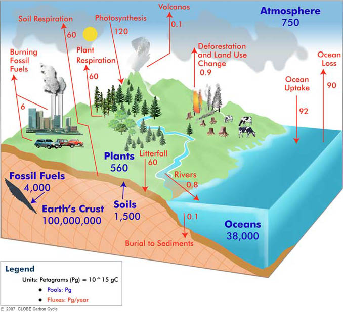
This simulation only includes carbon storage in the shallow oceans, in the atmosphere, in soil and in plants. The amounts stored are indicated graphically in the model by the sizes of the sea, cloud, soil (the brown rectangle) and the trees respectively. All stores supply carbon to the atmosphere but the ocean only receives carbon from the atmosphere and by run-off from the land (i.e. the soil), plants only receive carbon from the atmosphere and soil only gets its carbon from plants. All other fluxes are assumed to be small or zero.

On longer time scales other stores become very important because they are huge (see the illustration above which shows the Earth’s crust holding 100 million Gt of carbon). For example, a great deal of carbon is stored on the sea floor in the form of limestone and organic-rich shales. This material can, in turn, become subducted at ocean trenches into the deep Earth where it can be stored for millions of years before being re-emitted into the atmosphere through volcanoes. Some of this long-term carbon is also now being re-emitted into the atmosphere by human activities; oil is produced when organic-rich shales are buried and heated up over millions of years.
Is this the long-term or the short-term carbon cycle?
The model only simulates the short-term carbon-cycle, i.e. changes that can occur on timescales of a few years. You can see the lengths of time involved by looking at the Lifetimes display. The main difference, between this short-term simulation and a model including longer-term processes, is that the program you are using here does not include carbon-storage in the deep-ocean, in ocean sediments and in the interior of the Earth. These stores operate on timescales as high as several million years and will not influence changes in, for example, atmospheric CO2 levels on human timescales.
How does carbon move between the atmosphere and the ocean ?
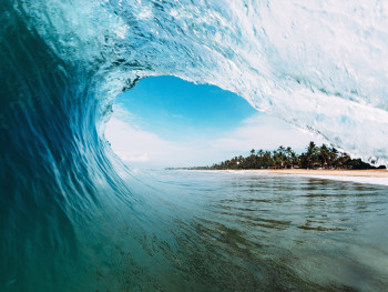
This is a complex process not yet fully understood. Some carbon dioxide is absorbed by rainfall (which makes the rain slightly acidic) and this either falls directly onto the sea or falls onto land where it can chemically react with rocks to produce carbon-bearing chemicals in rivers. However, most of the exchange happens directly at the sea-surface where CO2 can diffuse into or out of the ocean (depending on the relative concentrations in the water and air). This process is faster when there are waves and so it depends strongly on the wind-speed.
What is Gt short for?
Gt is an abbreviation for Gigatonne. One metric tonne is 1000 kg and a gigatonne is 1 billion ( 1 000 000 000 ) tonnes.
What is Exponential Decay?
The best known example of exonential decay is probably the “half-life” of a radioactive element. For example, the half-life of Carbon-14 (the element used in radioocarbon dating) is 5730 years. This means that, after 5730 years, half of the Carbon-14 that was present has changed into Nitrogen-14. After a further 5730 years, half of the remaining Carbon-14 will then decay, and so on. Note that this means the rate of loss of Carbon-14 slows down with time in such a way that there is always some left (see figure).
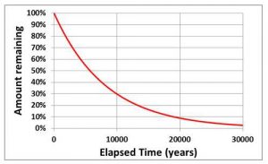
The stores in the carbon cycle model behave in a similar way so that, if you change a flux, the masses in the stores adjusts by “exponential decay” which means that they initially move rapidly towards the final equilibrium value but, as they approach it, the rate of change slows down. The lifetimes given in the carbon-cycle model are the times taken for about 2/3 of the change to occur and so these are slightly longer than “half-lives”. If you’re interested in knowing the half-lives, divide the lifetimes by 1.44 (e.g. a lifetime of 3000 years is equivalent to a half-life of 2079 years).